You know what though? Sometimes it's good to explore things that don't have an obvious business use case. Things that are weird. Things that are pretty. Things that are ridiculous. Things like dynamical systems and chaos. And, if you happen to find there are applicable tidbits along the way (*hint, skip to the problem outline section*), great, otherwise just enjoy the diversion.
motivation
So what is a dynamical system? Dryly, a dynamical system is a fixed rule to describe how a point moves through geometric space over time. Pretty much everything that is interesting can be modeled as a dynamical system. Population, traffic flows, fireflies, and neurons can all be describe this way.
In most cases, you'll have a system of ordinary differential equations like this:
\begin{eqnarray*}
\dot{x_{1}} & = & f_{1}(x_{1},\ldots,x_{n})\\
\vdots\\
\dot{x_{n}} & = & f_{n}(x_{1},\ldots,x_{n})
\end{eqnarray*}
In most cases, you'll have a system of ordinary differential equations like this:
For example, the Fitzhugh-Nagumo model (which models a biological neuron being zapped by an external current):
\begin{eqnarray*} \dot{v} & = & v-\frac{v^{3}}{3}-w+I_{{\rm ext}}\\ \dot{w} & = & 0.08(v+0.7-0.8w) \end{eqnarray*}
In this case \(v\) represents the potential difference between the inside of the neuron and the outside (membrane potential), and \(w\) corresponds to how the neuron recovers after it fires. There's also an external current \(I_{{\rm ext}}\) which can model other neurons zapping the one we're looking at but could just as easily be any other source of current like a car battery. The numerical constants in the system are experimentally derived from looking at how giant squid axons behave. Basically, these guys in the 60's were zapping giant squid brains for science. Understand a bit more why I think your business use case is boring?
One of the simple ways you can study a dynamical system is to see how it behaves for a wide variety of parameter values. In the Fitzhugh-Nagumo case the only real parameter is the external current \(I_{{\rm ext}}\). For example, for what values of \(I_{{\rm ext}}\) does the system behave normally? For what values does it fire like crazy? Can I zap it so much that it stops firing altogether?
In order to do that you'd just decide on some reasonable range of currents, say \((0,1)\), break that range into some number of points, and simulate the system while changing the value of \(I_{{\rm ext}}\) each time.
chaos
There's a a lot of great ways to summarize the behavior of a dynamical system if you can simulate its trajectories. Simulated trajectories are, after all, just data sets. The way I'm going to focus on is calculation of the largest lyapunov exponent. Basically, all the lyapunov exponent says is, if I take two identical systems and start them going at slightly different places, how similarly do they behave?
For example, If I hook a car battery to two identical squid neurons at the same time, but one has a little bit of extra charge on it, does their firing stay in sync forever or do they start to diverge in time? The lyapunov exponent would measure the rate at which they diverge. If the two neurons fire close in time but don't totally sync up then the lyapunov exponent would be zero. If they eventually start firing at the same time then the lyapunov exponent is negative (they're not diverging, they're coming together). Finally, if they continually diverge from one another then the lyapunov exponent is positive.
As it turns out, a positive lyapunov exponent usually means the system is chaotic. No matter how close two points start out, they will diverge exponentially. What this means in practice is that, while I might have a predictive model (as a dynamical system) of something really cool like a hurricane, I simply can't measure it precisely enough to make a good prediction of where it's going to go. A really small measurement error, between where the hurricane actually is and where I measure it to be, will diverge exponentially. So my model will predict the hurricane heading into Texas when it actually heads into Louisanna. Yep. Chaos indeed.
problem outline
So I'm going to compute the lyapunov exponent of a dynamical system for some range of parameter values. The system I'm going to use is the Henon Map:
\begin{eqnarray*}x_{n+1} & = & y_{n}+1-ax_{n}^{2}\\y_{n+1} & = & bx_{n}\end{eqnarray*}
I choose the Henon map for a few reasons despite the fact that it isn't modeling a physical system. One, it's super simple and doesn't involve time at all. Two, it's two dimensional so it's easy to plot it and take a look at it. Finally, it's only got two parameters meaning the range of parameter values will make up a plane (and not some n-dimensional hyperspace) so I can make a pretty picture.
What does Hadoop have to do with all this anyway? Well, I've got to break the parameter plane (ab-plane) into a set of coordinates and run one simulation per coordinate. Say I let \(a=[a_{min},a_{max}]\) and \(b=[b_{min},b_{max}]\) and I want to look \(N\) unique \(a\) values and \(M\) unique \(b\) values. That means I have to run \(N \times M\) individual simulations!
Clearly, the situation gets even worse if I have more parameters (a.k.a a realistic system). However, since each simulation is independent of all the other simulations, I can benefit dramatically from simple parallelization. And that, my friends, is what Hadoop does best. It makes parallelization trivially simple. It handles all those nasty details (which distract from the actual problem at hand) like what machine gets what tasks, what to do about failed tasks, reporting, logging, and the whole bit.
So here's the rough idea:
- Use Hadoop to split the n-dimensional (2D for this trivial example) space into several tiles that will be processed in parallel
- Each split of the space is just a set of parameter values. Use these parameter values to run a simulation.
- Calculate the lyapunov exponent resulting from each.
- Slice the results, visualize, and analyze further (perhaps at higher resolution on a smaller region of parameter space), to understand under what conditions the system is chaotic. In the simple Henon map case I'll make a 2D image to look at.
implementation
Hadoop has been around for a while now. So when I implement something with Hadoop you can be sure I'm not going to sit down and write a java map-reduce program. Instead, I'll use Pig and custom functions for pig to hijack the Hadoop input format functionality. Expanding the rough idea in the outline above:
- Pig will load a spatial specification file that defines the extent of the space to explore and with what granularity to explore it.
- A custom Pig LoadFunc will use the specification to create individual input splits for each tile of the space to explore. For less parallelism than one input split per tile it's possible to specify the number of total splits. In this case the tiles will be split mostly evenly among the input splits.
- The LoadFunc overrides Hadoop classes. Specifically: InputFormat (which does the work of expanding the space), InputSplit (which represents the set of one or more spatial tiles), and RecordReader (for deserializing the splits into useful tiles).
- A custom EvalFunc will take the tuple representing a tile from the LoadFunc and use its values as parameters in simulating the system and computing the lyapunov exponent. The lyapunov exponent is the result.
And here is the pig script:
define LyapunovForHenon sounder.pig.chaos.LyapunovForHenon();

points = load 'data/space_spec' using sounder.pig.points.RectangularSpaceLoader();

exponents = foreach points generate $0 as a, $1 as b, LyapunovForHenon($0, $1);

store exponents into 'data/result';
You can take a look at the detailed implementations of each component on github. See: LyapunovForHenon, RectangularSpaceLoader
running
$: cat data/space_spec
0.6,1.6,800
-1.0,1.0,800
Remember the system?
\begin{eqnarray*}x_{n+1} & = & y_{n}+1-ax_{n}^{2}\\y_{n+1} & = & bx_{n}\end{eqnarray*} Well, the spatial specification says (if I let the first line represent \(a\) and the second be \(b\)) that I'm looking at an \(800 \times 800\) (or 640000 independent simulations) grid in the ab-plane where \(a=[0.6,1.6]\) and \(b=[-1.0,1.0]\)
Now, these bounds aren't arbitrary. The Henon attractor that most are familiar with (if you're familiar with chaos and strange attractors in the least bit) occurs when \(a=1.4\) and \(b=0.3\). I want to ensure I'm at least going over that case.
result
$: cat data/result/part-m* | head
0.6	-1.0	9.132244649409043E-5
0.6	-0.9974968710888611	-0.0012539625419929572
0.6	-0.9949937421777222	-0.0025074937591903013
0.6	-0.9924906132665833	-0.0037665150764570965
0.6	-0.9899874843554444	-0.005032402237514987
0.6	-0.9874843554443055	-0.006299127065420516
0.6	-0.9849812265331666	-0.007566751054452304
0.6	-0.9824780976220276	-0.008838119048229768
0.6	-0.9799749687108887	-0.010113503950504331
0.6	-0.9774718397997498	-0.011392710785045064
$: cat data/result/part-m* > data/henon-lyapunov-ab-plane.tsv
To visualize I used this simple python script to get:
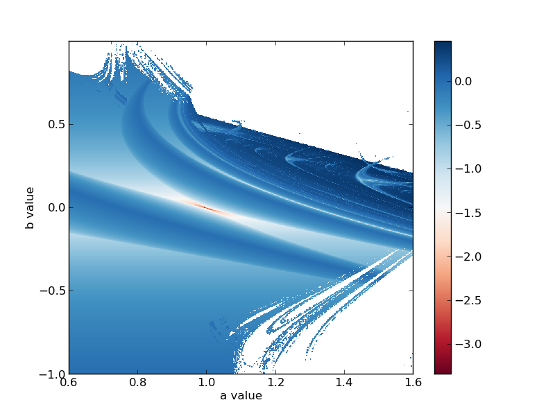
The big swaths of flat white are regions where the system becomes unbounded. It's interesting that the bottom right portion has some structure to it that's possibly fractal. The top right portion, between \(b=0.0\) and \(b=0.5\) and \(a=1.0\) to \(a=1.6\) is really the only region on this image that's chaotic (where the exponent is non-negative and greater than zero). There's a lot more structure here to look at but I'll leave that to you. As a followup it'd be cool to zoom in on the bottom right corner and run this again.
conclusion
So yes, it's possible to use Hadoop to do massively parallel scientific computing and avoid the question of big data entirely. Best of all it's easy.
The notion of exploding a space and doing something with each tile in parallel is actually pretty general and, as I've shown, super easy to do with Hadoop. I'll leave it to you to come up with your own way of applying it.