In fact, I'm going to assume just that. That you've used linear regression in other contexts before and understand its utility. The issue at hand is how to parallelize linear regression. Why? Well, suppose you have billions of feature vectors in your data set, each with thousands of features (columns), and you want to use all of them because, why not? Suppose it doesn't fit on one machine. Now, there exists a project to address this specifically, vowpal wabbit, which you should most certainly check out, but that I'm not going to talk about. Instead, the idea is to use Apache Pig. The reason for implementing it with Pig, rather than using an existing tool, is mostly for illustration. Linear regression with pig brings up several design and implementation details that I believe you'll face when doing almost any reasonably useful machine learning at scale. In other words, how do I wire all this shit together?
Specifically, I'll address pig macros, python drivers, and using a whole relation as a scalar. Fun stuff.
linear regression
It's important that I do at least explain a bit of terminology so we're all together in this. So, rather than jump for the most general explanation immediately (why do people do that?) let's talk about something real. Suppose you've measured the current running through a circuit while slowly decreasing the resistance. You would expect the current to increase linearly as you decrease the current (ohms law). In other words,
\begin{eqnarray*}I=\frac{V}{R}\end{eqnarray*}
To verify Ohm's Law (not a bad idea, I mean, maybe you're living in a dream world where physics is different and you want to know for certain...) you'd record the current \(I\) and the resistance \(R\) at every measurement while holding the voltage \(V\) constant. You'd then fit a line to the data or, more specifically, to \(\frac{1}{R}\), and, if all went well, find that the slope of said line was equal to the voltage.
In the machine learning nomenclature the current would be called the response or target variable. All the responses together form a vector \(y\) called the response vector. The resistance would be called the feature or observation. And, if you recorded more than just the resistance, say, the temperature, then for every response you'd have a collection of features or a feature vector. All the feature vectors together form a matrix \(X\). The goal of linear regression is to find the best set of weights \(w\) that, when used to form a linear combination of the features, creates a vector that is as close as possible to the response vector. So the problem can be phrased as an optimization problem. Here the function we'll minimize is the mean squared error (the square of the distance between the weighted features and the response). Mathematically the squared error, for one feature vector \(x_{i}\) of length \(M\), can be written as:
\begin{eqnarray*}error^2=(y_{i}-\sum_{j=1}^Mw_{j}x_{i,j})^2\end{eqnarray*}
where \(x_{i,0}=1\) by definition.
So the mean squared error (mse), when we've got \(N\) measurements (feature vectors), is then:
\begin{eqnarray*}mse(w)=\frac{1}{N}\sum_{i=1}^N(y_{i}-\sum_{j=1}^Mw_{j}x_{i,j})^2\end{eqnarray*}
So now the question is, exactly how are we going to minimize the mse by varying the weights? Well, it turns out there's the method called gradient descent. That is, the mse decreases fastest if we start with a given set of weights and travel in the direction of the negative gradient of the mse for those weights. In other words:
\begin{eqnarray*}w_{new}=w-\alpha\nabla{mse(w)}\end{eqnarray*}
Where \(\alpha\) is the magnitude of the step size. What this gives us is a way to update the weights until \(w_{new}\) doesn't really change much. Once the weights converge we're done.
algorithm
Alright, now that we've got a rule for updating weights, we can write down the algorithm.
1. Initialize the weights, one per feature, randomly
1. Initialize the weights, one per feature, randomly
2. Update the weights by subtracting the gradient of the mse
3. Repeat 2 until converged
implementation
Ok great. Let's get the pieces together.
pig
Pig is going to do most of the real work. There's two main steps involved. The first step, and one that varies strongly from domain to domain, problem to problem, is loading your data and transforming it into something that a generic algorithm can handle. The second, and more interesting, is the implementation of gradient descent of the mse itself.Here's the implementation of the gradient descent portion. I'll go over each relation in detail.
Go ahead and save that in a directory called 'macros'. Since gradient descent of the mean squared error for the purposes of creating a linear model is a generic problem, it makes sense to implement it as a pig macro.
In lines 19-25 we're attaching the weights to every feature vector. The Zip UDF, which can be found on github, receives the weights as a tuple and the feature vector as a tuple. The output is a bag of new tuples which contains (weight,feature,dimension). Think of Zip like a zipper where it matches the weights to their corresponding features. Importantly, the dimension (index in the input tuples) is returned as well.
Something to notice about this first bit is the scalar cast. Zip receives the entire weights relation as a single object. Since the weights relation is only a single tuple anyway, this is great. This is a good thing. It prevents us from doing something silly like a replicated join on a constant (which works but clutters the logic) or, worse, a cross.
Next, in lines 32-39, we're computing a portion of the gradient of the mse. The reason for the Zip udf in the first step was so the nested projection and sum to compute the dot product of the weights with the features works out cleanly.
Then, on line 42, the full gradient of the mse is computed by multiplying each feature by the error. It might not seem obvious when written like that, but the partial derivatives of the mse with respect to each weight make it work out like this. How nice.
Lines 47-54 is where the action happens. By action I mean we'll actually trigger a reduce job since everything up to this point has been map only. This is where the partial derivative bits come together. That is, we're grouping by dimension and weight (which, it turns out is precisely the thing we're differentiating with respect to) and summing each feature vector's contribution to the partial derivative along that dimension. The factor bit, on line 48, is the multiplier for the gradient. It includes the normalization term (we normalize by the number of features since we're differentiating the mean squared error) and the step size. The result of this step is a new weight for each dimension.
An important thing to note here is that there are only a number of partitions equivalent to the number of features. What this means is that each reduce task would get a potentially very large amount of data. Fortunately for us COUNT and SUM are both algebraic and so Pig will use combiners, hurray!, drastically reducing the amount of data sent to each reduce task.
Finally, on lines 60-65, we reconstruct a new tuple with the new weights and return it. The schema of this tuple should be the same as the input weight tuple.
gory details
So now that we have a way to do it, we should do it. Right, I mean if we can we should. Isn't that how technology works...
I'll going to go ahead and do a completely contrived example. The reason is so that I can visualize the results.
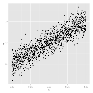
I've created some data, called data.tsv, which satisfies the following:
\begin{eqnarray*}y=0.3r(x) + 2x\end{eqnarray*}
where \(r(x)\) is a noise term. And here's the plot:
So we have two feature columns, (1.0, \(x\)), that we're trying to find the weights for. Since we've cooked this example (we already know the relationship between \(x\) and \(y\)) we expect the weights for those columns to be (0.0,2.0) if all goes well.
Now that we've got some data to work with, we'll need to write a bit more pig to load the data up and run it through our gradient descent macro.
The driver script is next. Since our algorithm is iterative and pig itself has no support for iteration, we're going to embed the pig script into a python (jython) program. Here's what that looks like:
There's a lot going on here (it's cluttered looking because Pig doesn't allow class or function definitions in driver scripts) that's not that interesting and pretty easy to understand so I'll just go over the high points:
- We initialize the weights randomly and write a .pig_schema file as well. The reason for writing the schema file is so that it's unnecessary to write the redundant schema for weights in the pig script itself.
- We want the driver to be agnostic to whether we're running in local mode or mapreduce mode. Thus we copy the weights to the filesystem using the copyFromLocal fs command. In local mode this just puts the initial weights on the local fs whereas in mapreduce mode this'll place them on the hdfs.
- Then we iterate until the convergence criteria is met. Each iteration details like copying the schema, and pulling down the weights to compute distances is done.
- A moving average is maintained over the past 25 weights. Iteration stops when the new weight is less than EPS away from the average.
Aside from that there's an interesting -bug?- that comes up as a result of this. Notice on line 70 how the new variables are bound each iteration? Well the underlying PigContext object just keeps adding these new variables instead of overwriting them. What this means is that, after a couple thousand iterations, depending on your PIG_HEAPSIZE env variable, the driver script will crash from an out of memory error. Yikes.
run it
Finally we get to run it. That part's easy:
$: export PIG_HEAPSIZE=4000
$: pig driver.py fit_line.pig data data.tsv 2
That is, we use the pig command to launch the driver program. The arguments to the driver script itself follow. We're running the fit_line.pig script where the data dir (where intermediate weights will go) exists under 'data' and the input data, data.tsv, should exist there as well. The '2' indicates we've got two weights (w0, and w1). The pig heapsize is to deal with the bug mentioned in the previous section.
On my laptop, in local mode, the convergence criteria was met after 1527 iterations.
results
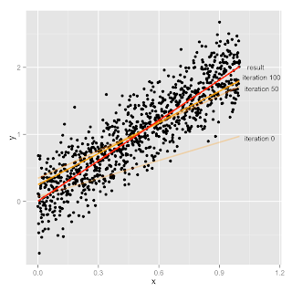
After 1527 iterations the weights ended up as (0.0040666759502969215, 2.0068029003414014) which is exactly what we'd expect. In other words:
\begin{eqnarray*}y=0.0041 + 2.0068x\end{eqnarray*}
which is the 'best fit' line to our original:\begin{eqnarray*}y=0.3r(x) + 2x\end{eqnarray*}
And here's an illustration of what happened.
Looks pretty reasonable to me. Hurray. Now go fit some real data.

